
Website Traffic Forecasting refers to predicting website traffic for a specific period. It is one of the most effective applications of Time Series Forecasting. If you want to learn how to forecast website traffic, this article is for you. In this article, we will guide you through the process of Website Traffic Forecasting using Python.
Website Traffic Forecasting Using Python
The dataset we are using for Website Traffic Forecasting is collected from the daily traffic data of XYZ site.. It contains records of daily website visits over the past 12 months.
Now, let’s begin the website traffic forecasting task by importing the required Python libraries and loading the dataset:
from google.colab import drive
drive.mount('/content/drive')

import pandas as pd
import numpy as np
import matplotlib.pyplot as plt
import matplotlib.dates as mdates
import statsmodels.api as sm
from statsmodels.tsa.statespace.sarimax import SARIMAX


file_id="1mFWURXYZS_JZUeiemVDDE_IdzglnTrEF"
url=f"https://drive.google.com/uc?id={file_id}"

data=pd.read_csv(url)
print(data.head())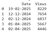
Lets check the data type of Date column.
data.info()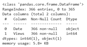
As the date column is currently stored as an object type, we will first convert it into a datetime type before proceeding further.
data['Date'] = pd.to_datetime(data['Date'], format="%d-%m-%Y")data.info()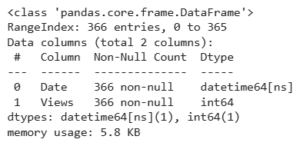
As we can see the date is not sorted, lets sort the date and make the columns as index. Setting the Date column as the index makes the dataset time-aware, ensuring accurate plotting, resampling, and properly aligned forecasts.
data = data.sort_values('Date').set_index('Date')
data.head(20)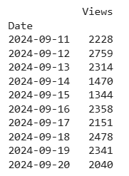
Now, let’s examine the website’s daily traffic
plt.style.use('fivethirtyeight')
plt.figure(figsize=(15, 10))
plt.plot(data["Views"])
plt.title("Daily Traffic of XYZ")
plt.show()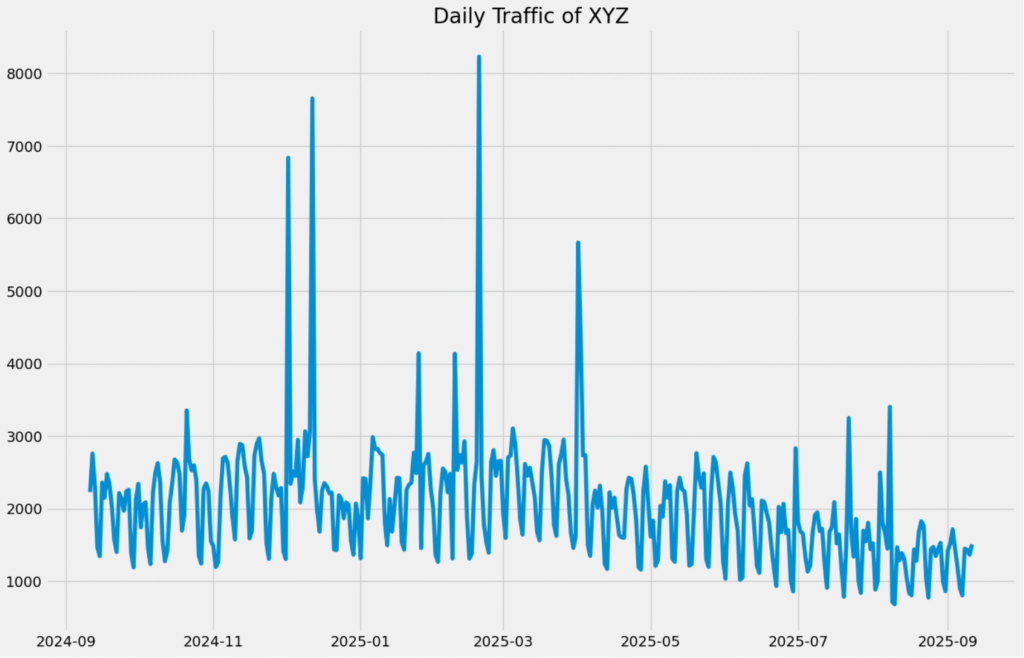
Observations: Overall Pattern: The traffic fluctuates daily with a repeating up-down rhythm → this suggests weekly seasonality (higher traffic on some weekdays, lower on weekends).
Traffic Spikes: Noticeable sharp spikes (Nov 2024, Dec 2024, Mar 2025) → these are likely due to campaigns, product launches, or external promotions. The biggest spike occurs around March 2025, crossing 8,000+ views.
Trend: From Sep 2024 → Mar 2025: traffic is relatively high with several peaks. After April 2025, the traffic shows a gradual decline, with fewer high spikes and lower daily averages.
Seasonality: The sawtooth pattern suggests consistent weekly cycles (possibly business days vs. weekends). But the amplitude of fluctuations reduces after mid-2025, meaning fewer big surges.
Insights
- XYZ had strong campaigns or events driving spikes in late 2024 and early 2025.
- After March 2025, there’s a downward trend in daily traffic, which could signal reduced marketing efforts, lower organic reach, or seasonality effects.
- Weekly cycles are clear → marketing/content should be timed with high-traffic weekdays for maximum impact
Now, let’s examine whether our dataset exhibits stationarity or seasonality:
decomposition = seasonal_decompose(daily_views["Views"], model="multiplicative", period=30)
fig = decomposition.plot()
plt.show()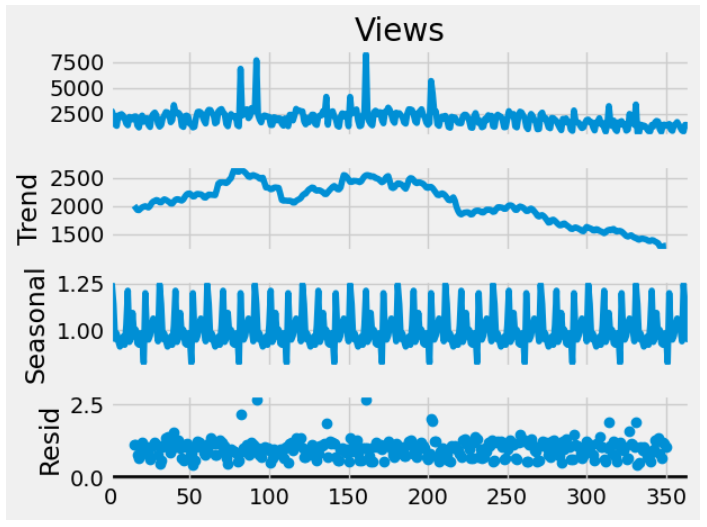
The seasonal decomposition of the website traffic reveals several important patterns. The observed series shows daily fluctuations with notable spikes around days 80, 120, 150, and 200, which are likely caused by specific events such as campaigns or content launches rather than regular behavior. The trend component indicates that traffic initially increased from around 1,800 views to nearly 2,500 but then declined steadily after approximately day 150, suggesting a slowdown in performance possibly linked to reduced campaigns, SEO changes, or seasonal effects.
The seasonal component highlights a strong and consistent weekly cycle, with traffic peaking on certain weekdays and dipping on others, confirming clear weekly seasonality. Finally, the residual component captures mostly small variations, though some large outliers remain, aligning with the sharp spikes observed in the raw data. Overall, the analysis confirms that the website traffic is both seasonal and event-driven, with a distinct weekly cycle, a growth-to-decline trend shift, and irregular surges tied to special promotions or campaigns.
We will be using the Seasonal ARIMA (SARIMA) model to forecast traffic on the website. Before applying the SARIMA model, it is necessary to determine the p, d, and q values. You can learn how to find p, d, and q values from here.
As the data is not stationary, the value of d is 1. To find the values of p and q, we can use the autocorrelation and partial autocorrelation plots:
pd.plotting.autocorrelation_plot(data["Views"])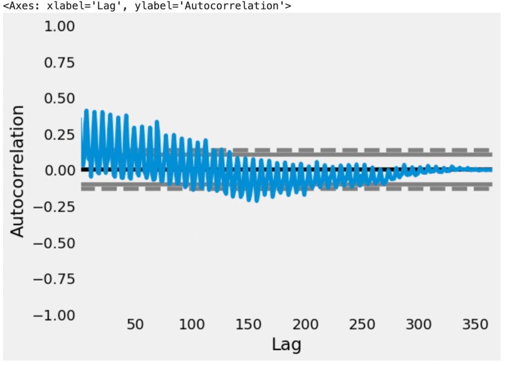
plot_pacf(data["Views"], lags = 100)
plt.show()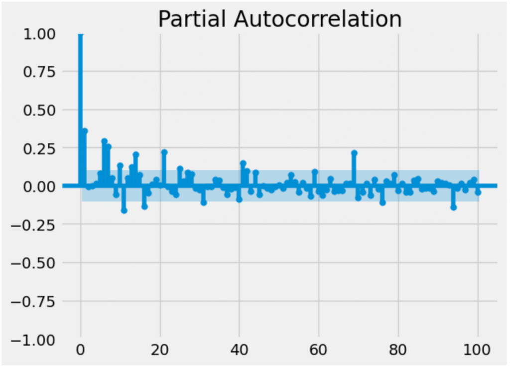
Website Traffic Forecast Model
Now let’s see how we can train a SARIMA model to forecast website traffic:
p, d, q = 5, 1, 2
model=sm.tsa.statespace.SARIMAX(data['Views'],
                                order=(p, d, q),
                                seasonal_order=(p, d, q, 12))
model=model.fit()
print(model.summary())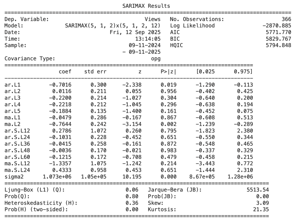
Website Traffic Forecasting
Now let’s forecast the website traffic for the next 50 days:
predictions = model.predict(len(data), len(data)+50)
print(predictions)
2025-09-12 1099.970651 2025-09-13 1273.874372 2025-09-14 1127.107085 2025-09-15 1049.435861 2025-09-16 1308.218615 2025-09-17 1311.187835 2025-09-18 1197.870811 2025-09-19 1173.982165 2025-09-20 1143.158734 2025-09-21 1155.060943 2025-09-22 1212.084809 2025-09-23 1182.583210 2025-09-24 1092.914702 2025-09-25 1492.266146 2025-09-26 1118.013164 2025-09-27 1004.576766 2025-09-28 1169.301282 2025-09-29 1121.362332 2025-09-30 1068.638220 2025-10-01 1153.948492 2025-10-02 1242.543474 2025-10-03 991.852202 2025-10-04 1085.850311 2025-10-05 1080.009573 2025-10-06 965.155899 2025-10-07 1172.886023 2025-10-08 1195.996716 2025-10-09 1087.043521 2025-10-10 1105.083410 2025-10-11 1002.615815 2025-10-12 979.594675 2025-10-13 1021.452858 2025-10-14 1222.467342 2025-10-15 1105.772794 2025-10-16 1123.477656 2025-10-17 1025.851038 2025-10-18 875.550440 2025-10-19 1211.808443 2025-10-20 1034.022184 2025-10-21 943.595163 2025-10-22 1089.265855 2025-10-23 977.996178 2025-10-24 883.531477 2025-10-25 885.881668 2025-10-26 1114.461008 2025-10-27 1024.634868 2025-10-28 998.747312 2025-10-29 1019.752299 2025-10-30 846.813576 2025-10-31 1211.240958 2025-11-01 952.707537 Freq: D, Name: predicted_mean, dtype: float64
Now let’s plot the forecasted values:
data["Views"].plot(legend=True, label="Training Data",
                   figsize=(15, 10))
predictions.plot(legend=True, label="Predictions")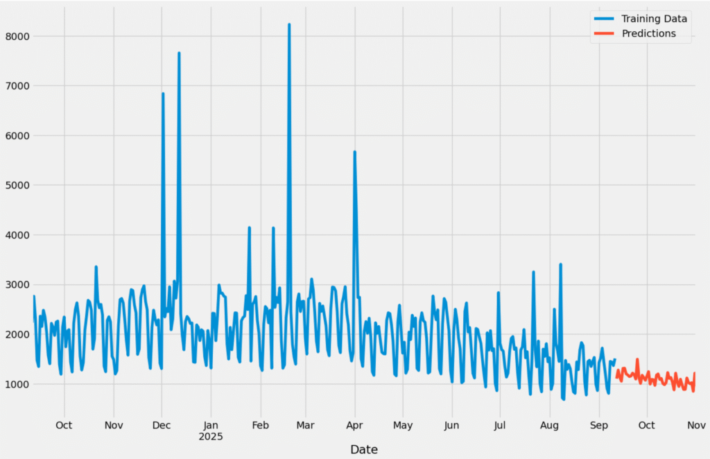
Conclusion
In conclusion, forecasting website traffic using a Seasonal ARIMA (SARIMA) model is a powerful method for anticipating future demand and helping guide strategic decisions — whether for server provisioning, content planning, or marketing campaigns. By first checking stationarity and differencing the data as needed, selecting the p, d, q (and seasonal P, D, Q) parameters via autocorrelation and partial autocorrelation plots, and then training the SARIMA model, we can generate reliable predictions. Visualizing the forecast and comparing it to actual traffic data helps validate the model and refine parameters. With a well-fitted SARIMA model, we can forecast traffic for the next 50 days (or whatever horizon is relevant), giving the business or website-owner a valuable forward-looking view that can improve resource planning and decision-making.