
By analyzing Uber trips, we can draw many patterns such as which day has the highest and the lowest trips, the busiest hour for Uber, and several other insights. The dataset we are using here is based on Uber trips from New York, a city with a very complex transportation system and a large residential community.
The dataset contains around 4.5 million Uber pickups in New York City from April to September and 14.3 million pickups from January to June 2015. There is so much more we can do with this dataset beyond simple analysis. But for now, in the section below, we will take you through Uber trips analysis using Python.
Uber Trips Analysis using Python
We will begin our Uber trips analysis by importing the necessary Python libraries and loading the dataset:
from google.colab import drive
drive.mount('/content/drive')

import pandas as pd
import matplotlib.pyplot as plt
import seaborn as sns

file_id="1tMXNuiASxHDaZsT8qmZ1Otqbov6H1oq1"
url=f"https://drive.google.com/uc?id={file_id}"

data=pd.read_csv(url)
data["Date/Time"]=data["Date/Time"].map(pd.to_datetime)
data.head()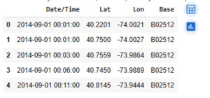
The dataset represents Uber trip pickups in New York City, with each row corresponding to a single trip. It includes four main columns: Date/Time, which records the exact timestamp of the pickup; Lat and Lon, which represent the latitude and longitude coordinates of the pickup location; and Base, a code identifying the Uber base or dispatching region from which the trip was assigned. Using this dataset, we can explore temporal patterns such as peak hours, daily and monthly trends, as well as geospatial insights like high-demand pickup hotspots across the city. Additionally, the base codes allow for analysis of trip distribution among different Uber bases, making this dataset a valuable resource for both time-series and location-based analysis.
For now, let’s prepare the dataset we are using to analyze Uber trips based on days and hours:
data["Day"]=data["Date/Time"].apply(lambda x:x.day)
data["Weekday"]=data["Date/Time"].apply(lambda x:x.weekday())
data["Hour"]=data["Date/Time"].apply(lambda x:x.hour)
data["Month"]=data["Date/Time"].apply(lambda x:x.month)
data.head()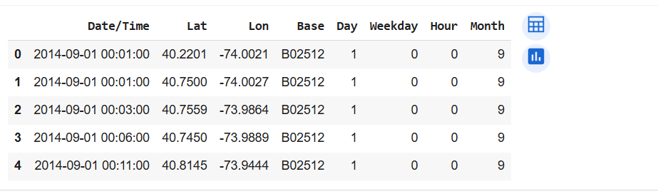
We have organized the data by days and hours, focusing on Uber trips for the month of September. Now, let’s examine each day to identify which day recorded the highest number of trips:
sns.set(rc={'figure.figsize':(12, 10)})
sns.distplot(data["Day"])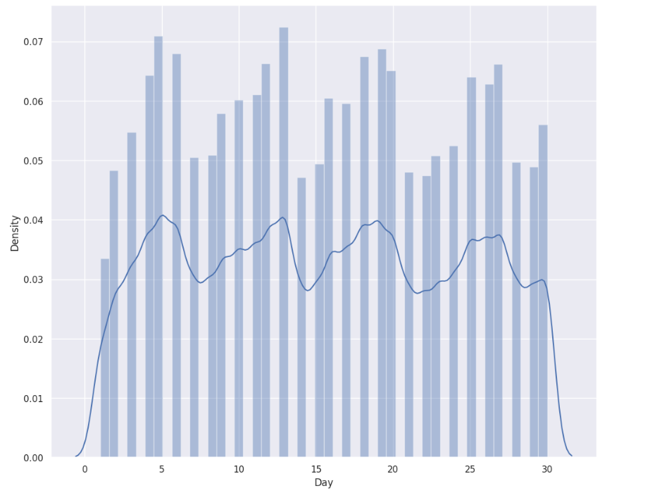
The plot shows Uber trip distribution across September, with steady activity throughout the month and noticeable peaks around the 5th, 15th, and 20th days. The trend line suggests a repeating weekly pattern, likely reflecting higher demand on specific weekdays or weekends.
Next, let’s analyze Uber trips based on hourly trends:
sns.distplot(data["Hour"])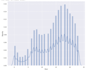
This plot illustrates the distribution of Uber trips across different hours of the day. The x-axis represents the hours (0–24), while the y-axis shows the density of trips. From the visualization, it’s clear that demand is relatively low during the early morning hours (midnight to around 5 AM). Activity gradually increases after 6 AM, reflecting morning commutes, and continues to rise through the day. The highest trip density occurs between 5 PM and 7 PM, aligning with evening rush hour when people are heading home from work. After that, trips remain high until around 9 PM before gradually declining late at night. Overall, the chart highlights strong daily patterns in Uber usage, with peak demand centered around commuting hours.
Next, let’s analyze Uber trips by weekdays:
sns.distplot(data["Weekday"])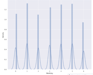
This plot shows the distribution of Uber trips across weekdays, where the x-axis represents days of the week (0 = Monday, 6 = Sunday) and the y-axis indicates trip density. The visualization highlights that Uber usage is fairly consistent on weekdays, with slightly higher activity on Tuesdays, Thursdays, and Fridays, which may be linked to mid- and end-of-week commuting or social activities. Weekends, especially Sundays, show relatively lower trip density compared to weekdays, suggesting reduced demand when fewer people are commuting for work. Overall, the data indicates that weekdays dominate Uber activity, while weekends see a noticeable dip.
Now, let’s explore how hours and weekdays together impact Uber trips:
# Correlation of Weekday and Hour
df=data.groupby(["Weekday", "Hour"]).apply(lambda x: len(x))
df=df.unstack()
sns.heatmap(df, annot=False)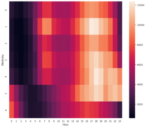
This heatmap shows the combined effect of hours and weekdays on Uber trip density. The x-axis represents hours of the day (0–23), and the y-axis represents weekdays (0 = Monday, 6 = Sunday). The color scale indicates trip volume, with darker shades showing lower activity and lighter shades showing higher activity.
From the visualization, we see that Uber demand is generally low in the early morning hours (midnight–5 AM) across all days. Starting around 6–9 AM, trips increase moderately, likely due to morning commutes. The highest concentration of trips consistently appears between 5 PM and 8 PM on weekdays, reflecting evening rush hours. Interestingly, weekends (Saturday and Sunday) show higher late-night activity compared to weekdays, suggesting demand from nightlife and social activities. Overall, the heatmap highlights two clear patterns: weekday peaks during commuting hours and weekend peaks during evenings and nights.
Since our dataset includes longitude and latitude, we can also plot the density of Uber trips across different regions of New York City:
data.plot(kind="scatter", x='Lon', y='Lat', alpha=0.4, s=data['Day'], label='Uber Trips',
figsize=(12, 8), cmap=plt.get_cmap('jet') )
plt.title("Uber Trips Analysis")
plt.legend()
plt.show()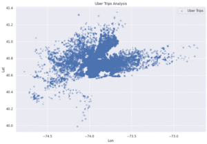
This scatter plot maps Uber trips across New York City using latitude (Lat) and longitude (Lon). Each point represents a pickup location, showing how trips are distributed geographically. The dense clusters of points highlight areas with the highest demand, particularly around central Manhattan, which appears as the darkest concentration. The spread of points toward surrounding regions such as Brooklyn, Queens, and parts of New Jersey indicates that while Uber is widely used across the metro area, Manhattan remains the core hotspot for activity. The plot also reveals sparser but noticeable trips extending to outer boroughs and nearby suburbs, showing Uber’s role in connecting both high-density urban centers and less-populated areas.
Conclusion
In summary, our analysis of Uber trip data in New York City reveals clear and consistent patterns. Demand is lowest during early morning hours (midnight to ~5 AM), increases steadily through the morning, and peaks in the early evening (around 5-7 PM), aligning with commuting times. Weekdays see higher usage overall than weekends, while select days such as Tuesday, Thursday, and Friday show especially strong activity. Geospatial plotting confirms Manhattan as the major hub of activity, with surrounding boroughs contributing more in peripheral areas. These insights can help inform drivers, service planners, and city transit authorities to better anticipate demand, optimize resource allocation, and improve urban mobility strategies. For a deeper dive into digital data trends, check out our Instagram Reach Analysis to explore how engagement patterns compare across platforms.