
Time Series Forecasting involves analyzing and modeling data collected over time to predict future outcomes. It has a wide range of applications, including weather prediction, sales projections, business planning, and stock price forecasting. One of the most widely used statistical methods for this purpose is the ARIMA model.
What is ARIMA?
ARIMA stands for AutoRegressive Integrated Moving Average. It’s a popular statistical method used to predict future values in a time series, like sales, temperature, or stock prices, based on past data.
The ARIMA model has three main parameters, written as ARIMA(p, d, q). Let’s understand what each one means:
p (autoregressive part): This tells the model how many past values (lags) it should look at when making a prediction. Example: If p = 2, the model will use the last 2 time points to help predict the next value.
d (integrated part): This tells the model how many times to difference the data to make it stable (or stationary). Stationary means the data doesn’t show trends or seasonal patterns, it stays around the same level over time. Example: If the data is already stable, d = 0. If it has trends or seasonality, d might be 1.
q (moving average part): This tells the model how many past error terms (differences between predicted and actual values) it should use to correct its predictions. Example: If q = 1, the model uses the last prediction error to improve the next forecast.
Time Series Forecasting Using ARIMA Model
Let’s begin the Time Series Forecasting task using the ARIMA model. To start, I’ll fetch Google’s stock price data using the Yahoo Finance API. First, you need to install yfinance API by using the pip command in your terminal or command prompt as mentioned below:
pip install yfinance
Now, let’s retrieve Google’s stock price data:
import pandas as pd
import yfinance as yf
import datetime
from datetime import date, timedelta
today=date.today()

d1 = today.strftime("%Y-%m-%d")
end_date=d1
d2=date.today()-timedelta(days=365)
d2=d2.strftime("%Y-%m-%d")
start_date=d2

data=yf.download('GOOG',
                start=start_date,
                end=end_date,
                progress=False)
data["Date"]=data.index
data=data[["Date", "Open","High", "Low", "Close", "Volume"]]
data.reset_index(drop=True, inplace=True)
data.tail()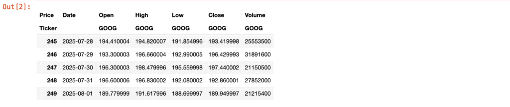
We only require the date and closing price for the remaining steps. Let’s select these two columns and proceed.
data=data[["Date", "Close"]]
data.head()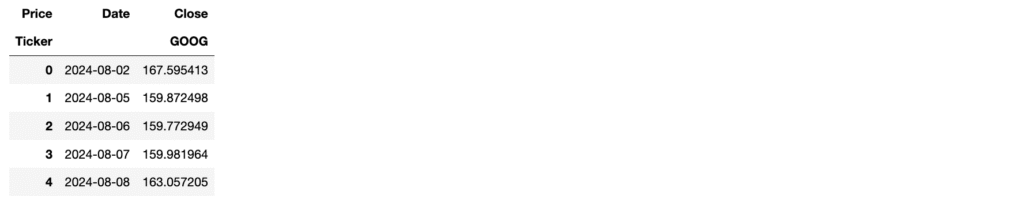
Let’s visualize Google’s closing stock prices before proceeding further.
import matplotlib.pyplot as plt
plt.style.use('fivethirtyeight')
plt.figure(figsize=(15, 10))
plt.plot(data["Date"], data["Close"]);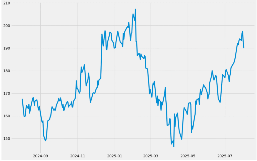
Forecasting Time Series Data with ARIMA
Before applying the ARIMA model, it’s important to determine whether the dataset is stationary or exhibits seasonality. The earlier visualization of closing stock prices indicates that the data is not stationary. To assess this more accurately, we can use seasonal decomposition, which breaks the time series into its trend, seasonal, and residual components. This helps provide a clearer understanding of the underlying patterns in the data before modeling.
from statsmodels.tsa.seasonal import seasonal_decompose
result= seasonal_decompose(data["Close"],
                           model='multiplicative',
                          period=30)
fig=plt.figure()
fig=result.plot()
fig.set_size_inches(15, 10)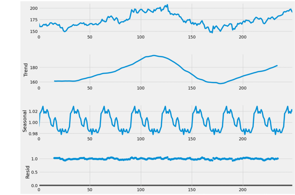
The decomposition plot shows that the Google stock price data has a clear upward and downward trend over time, along with a repeating seasonal pattern. This means the data is not stable (or stationary), as it changes over time and shows regular fluctuations. The seasonal pattern seems to repeat every month, and the leftover noise (residuals) appears random, which is a good sign.
Based on this, we can say that the data has both trend and seasonality. So, instead of using a basic ARIMA model, we should use a SARIMA model, which is better suited for data with seasonal behavior.
To apply ARIMA or SARIMA, we need to determine the values of p, d, and q. The p value can be identified using the partial autocorrelation plot of the Close prices, while the q value can be found using the autocorrelation plot. The d value is typically either 0 or 1, use 0 if the data is stationary and 1 if it’s seasonal. Since our dataset shows clear seasonality, we will use 1 as the value for d.
Here’s how to find the value of q:
pd.plotting.autocorrelation_plot(data["Close"])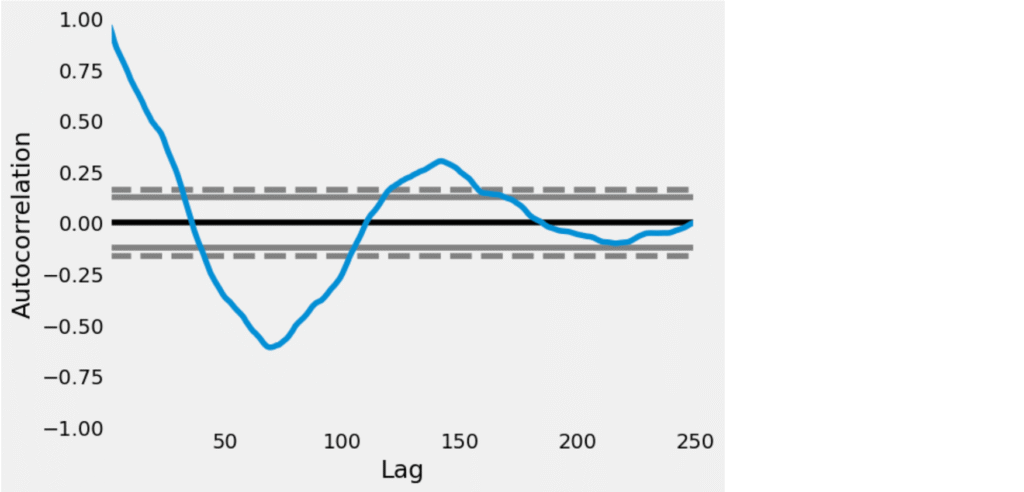
This is an Autocorrelation Function (ACF) plot, which helps in determining the q value (the number of Moving Average terms) for an ARIMA model.
How to interpret the ACF plot:
- x-axis (Lag): Number of lag periods (up to 250 here).
- y-axis (Autocorrelation): Degree of correlation between the time series and its lagged values.
- The dashed grey lines represent the 95% confidence interval.
- Significant lags are those where the autocorrelation goes beyond these confidence bands
Identifying the value of q:
- The first few lags (especially lag 1 and 2) are well outside the confidence interval.
- After around lag 2, the autocorrelation drops and starts oscillating, eventually staying mostly within the confidence band.
Conclusion:
- The ACF plot shows significant autocorrelation at lags 1 and 2, and then it decays.
- Therefore, the suggested value of q = 2.
Let’s find the value of p:
from statsmodels.graphics.tsaplots import plot_pacf
plot_pacf(data["Close"], lags=100)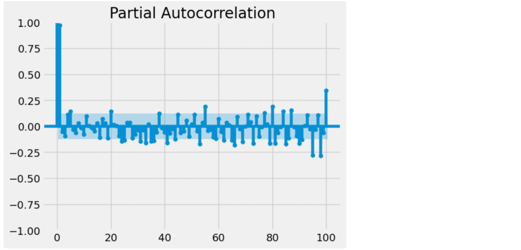
How to interpret the PACF plot:
- The x-axis shows the number of lags (1 to 100).
- The y-axis shows the partial autocorrelation coefficients.
- The blue shaded region indicates the confidence interval (typically 95%).
- Any bar outside this region is considered statistically significant.
Identifying the value of p:
- Lag 1 is clearly significant — the bar is well outside the confidence interval.
- From Lag 2 onward, all bars appear to be within the confidence interval, meaning they are not statistically significant.
- The PACF plot cuts off after lag 1.
- Therefore, the suggested value of p = 1.
Now let’s build an ARIMA model:
p, d, q= 1, 2, 1
from statsmodels.tsa.arima.model import ARIMA
model= ARIMA(data["Close"], order=(p,d,q))
fitted= model.fit()
print(fitted.summary())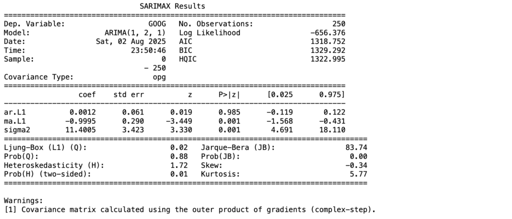
Here’s how you can make predictions using the ARIMA model:
predictions=fitted.predict()
print(predictions)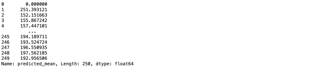
The predictions are inaccurate due to the seasonal nature of the data. Since ARIMA doesn’t account for seasonality, it’s not the best choice for this kind of time series. Lets check with SARIMA model.
So, here’s how to build a SARIMA model:
from statsmodels.tsa.statespace.sarimax import SARIMAX
import warnings
model=SARIMAX(data['Close'],
              order=(p, d, q),
              seasonal_order=(p, d, q, 12))
model=model.fit()
print(model.summary())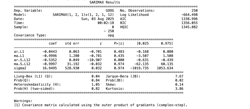
Now let’s predict the stock prices using the SARIMA model for the next 10 days:
predictions = model.predict(len(data), len(data)+10)
print(predictions)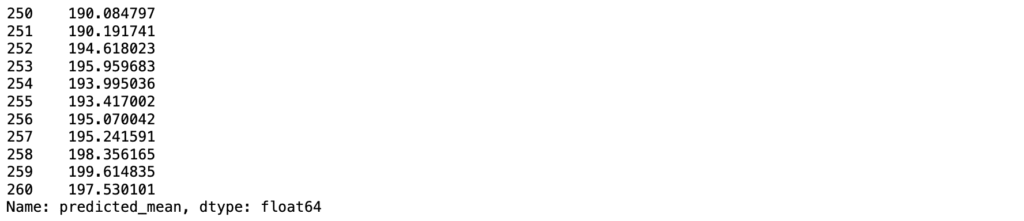
Now, let’s plot the predictions:
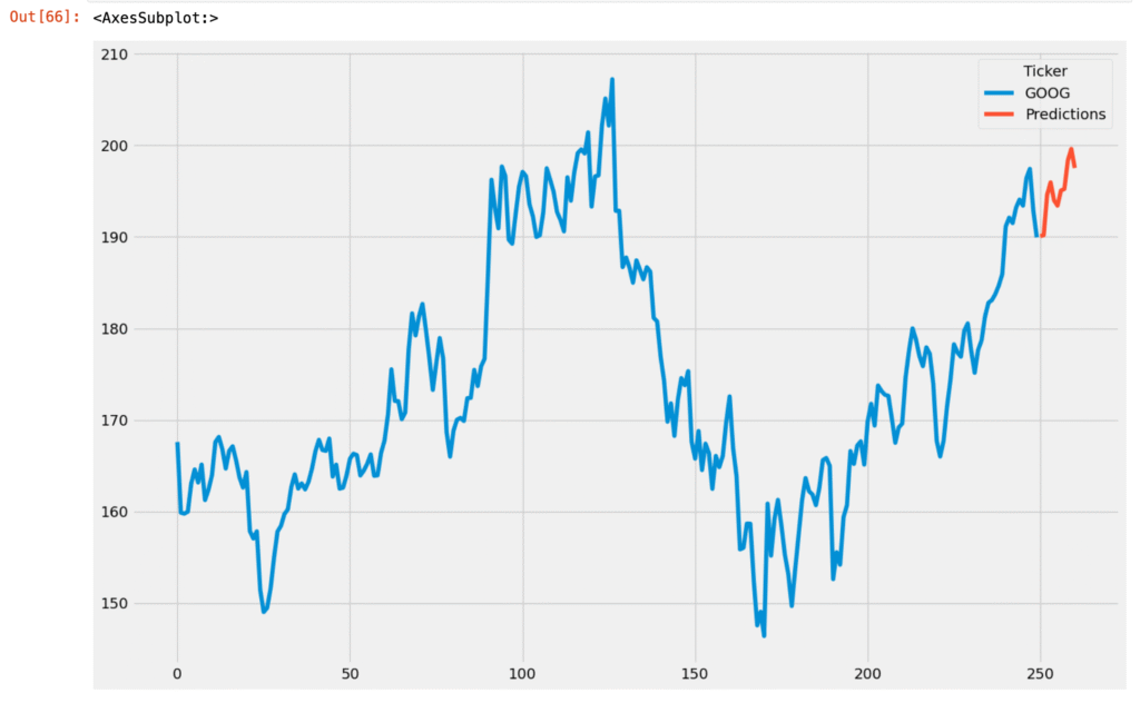
This is how you can apply ARIMA or SARIMA models for time series forecasting in Python.
Conclusion:
The ARIMA model serves as a robust statistical tool for time series forecasting, effectively capturing patterns in data to predict future trends. Its application spans various domains, including finance, sales, and weather forecasting. By understanding and correctly applying the ARIMA model, practitioners can make informed predictions that aid in strategic planning and decision-making. For those interested in implementing ARIMA in Python, the provided code snippets offer a practical starting point. Additionally, exploring related models like SARIMA can enhance forecasting accuracy, especially when dealing with seasonal data.