Banks and credit card companies rely on credit scores to assess a customer’s creditworthiness. A high credit score makes it easier for these institutions to approve loans and credit offers. Today, many financial institutions use machine learning algorithms to classify customers based on their credit history. If you’re interested in learning how to apply machine learning to credit score classification, this article will walk you through the process of building a credit score classification model using Python.
Credit Score Classification
Banks and credit card companies typically categorize customers into three credit score levels: Good, Standard, and Poor
Individuals with a good credit score are more likely to be approved for loans by financial institutions. To perform credit score classification using Machine Learning, we need a labelled dataset that reflects customers’ credit histories. I’ve found a suitable dataset that classifies credit card users based on their credit history. You can download it from here.
Let’s start credit score classification by importing the necessary Python libraries and the dataset:
import pandas as pd
import numpy as np
import plotly.express as px
import plotly.graph_objects as go
import plotly.io as pio
data=pd.read_csv("/Users/rahul_anand/Downloads/train.csv")
data.head()
pio.templates.default = "plotly_white"
Let’s explore the information about the columns in the dataset:
print(data.info())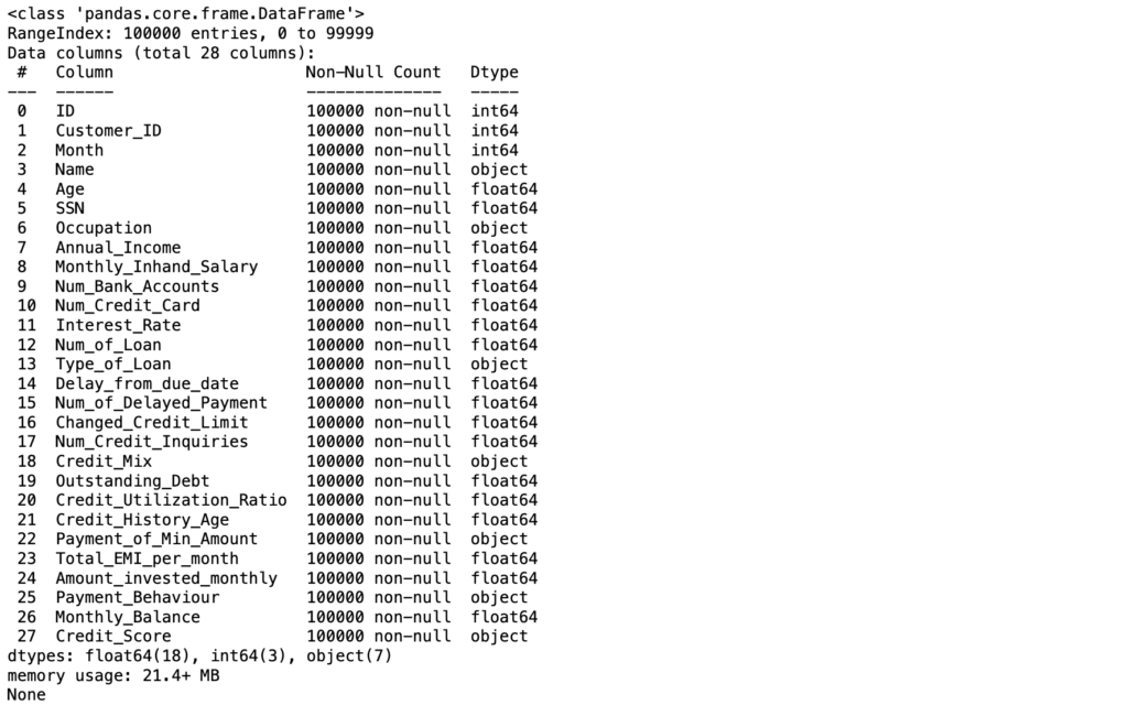
Before moving forward, let’s check whether the dataset has any null values or not:
print(data.isnull().sum())
* The dataset doesn’t have any null values.
As this dataset is labelled, let’s check the Credit_Score column values:
data["Credit_Score"].value_counts()
Exploratory Data Analysis
The dataset contains several features that can be used to train a Machine Learning model for credit score classifications. Let’s begin by checking each feature in detail.
An occupation feature to see whether a person’s profession has any impact on their credit score.
fig= px.box(data,
            x="Occupation",
            color='Credit_Score',
            title="Credit Scores Based on Occupation",
            color_discrete_map={'Poor': 'red', 'Standard':'yellow', 'Good':'Green'})
fig.show()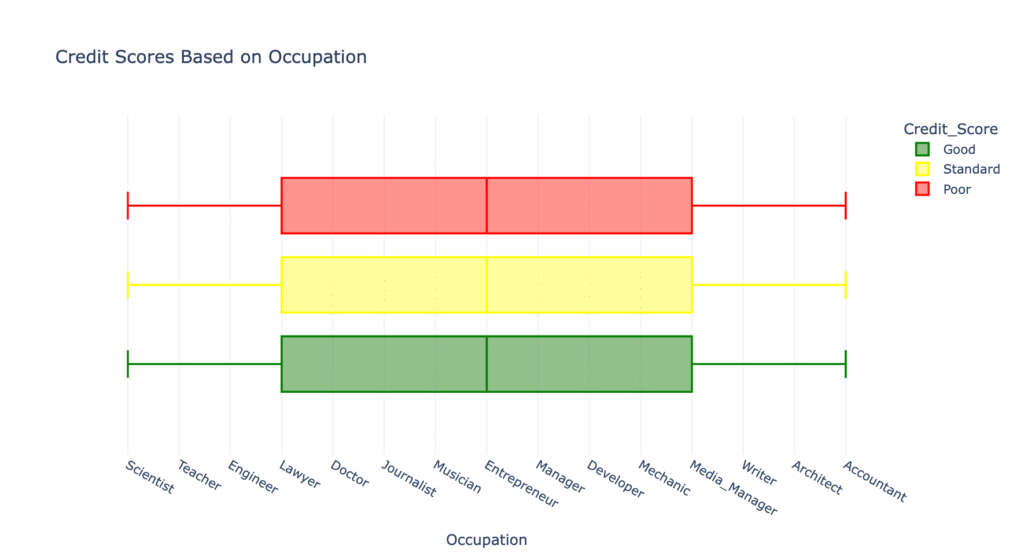
There’s not much difference in the credit scores of all occupations mentioned in the data.
Now, let’s explore whether the Annual Income of the person impacts your credit scores or not:
fig = px.box(data, x="Credit_Score", y="Annual_Income", color="Credit_Score", title="Credit Scores Based on Annual Income", color_discrete_map={'Poor':'red', 'Standard':'yellow', 'Good':'green'})
fig.update_traces(quartilemethod="exclusive")

fig.show()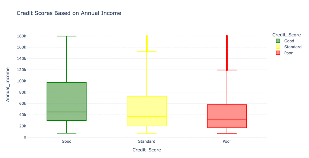
According to the above plot, the more you earn annually, the better your credit score is.
Now, let’s explore whether the monthly in-hand salary impacts credit scores or not:
fig=px.box(data, x="Credit_Score",
                 y="Monthly_Inhand_Salary",
                 color="Credit_Score",
                 title="Credit Scores Based on Monthly Inhand Salary",
           color_discrete_map={'Poor':'red',
                               'Standard':'yellow',
                               'Good':'green'})
fig.update_traces(quartilemethod="exclusive")
fig.show()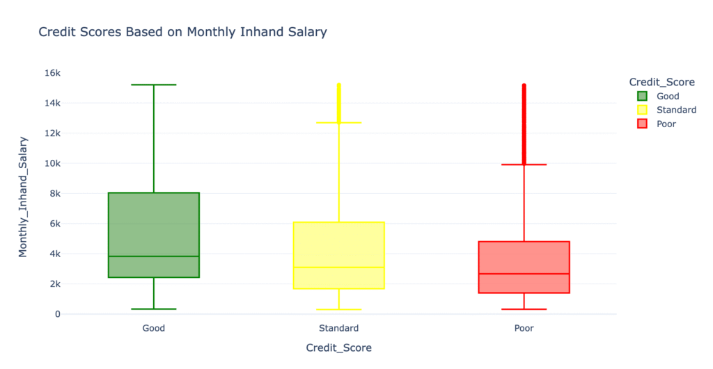
Like annual income, the more monthly in-hand salary you earn, the better your credit score will become.
Now let’s see if having more bank accounts impacts credit scores or not:
fig=px.box(data,
           x="Credit_Score",
           y="Num_Bank_Accounts",
           color="Credit_Score",
           title="Credit Scores Based on Number of Bank Accounts",
           color_discrete_map={'Poor':'red', 'Standard':'yellow', "Good":'green'})
fig.update_traces(quartilemethod="exclusive")
fig.show()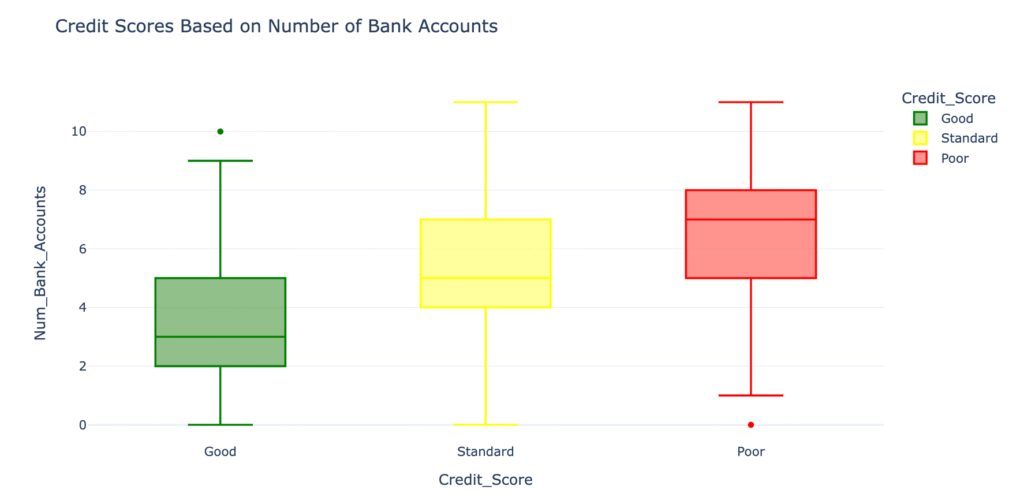
Maintaining more than five accounts is not good for having a good credit score. A person should have only 2 – 3 bank accounts. So having more bank accounts doesn’t positively impact credit scores.
Now, let’s see the impact on credit scores based on the number of credit cards you have:
fig = px.box(data,
             x="Credit_Score",
             y="Num_Credit_Card",
             color="Credit_Score",
             title="Credit Scores Based on Number of Credit cards",
             color_discrete_map={'Poor':'red',
                                 'Standard':'yellow',
                                 'Good':'green'})
fig.update_traces(quartilemethod="exclusive")
fig.show()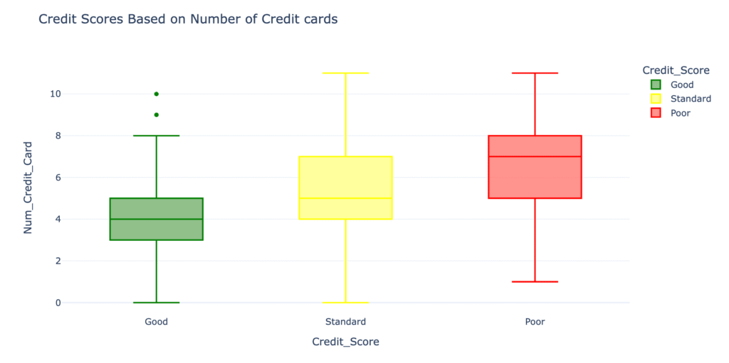
Just like the number of bank accounts, having more credit cards will not positively impact your credit scores. Having 3 – 5 credit cards is good for your credit score.
Now let’s see the impact on credit scores based on how much average interest you pay on loans and EMIs:
fig=px.box(data, x="Credit_Score",
           y="Interest_Rate",
           color="Credit_Score",
           title="Credit Scores Based on the Averge Interest rate",
           color_discrete_map={'Poor':'red',
                               'Standard':'yellow',
                               'Good':'green'})
fig.update_traces(quartilemethod="exclusive")
fig.show()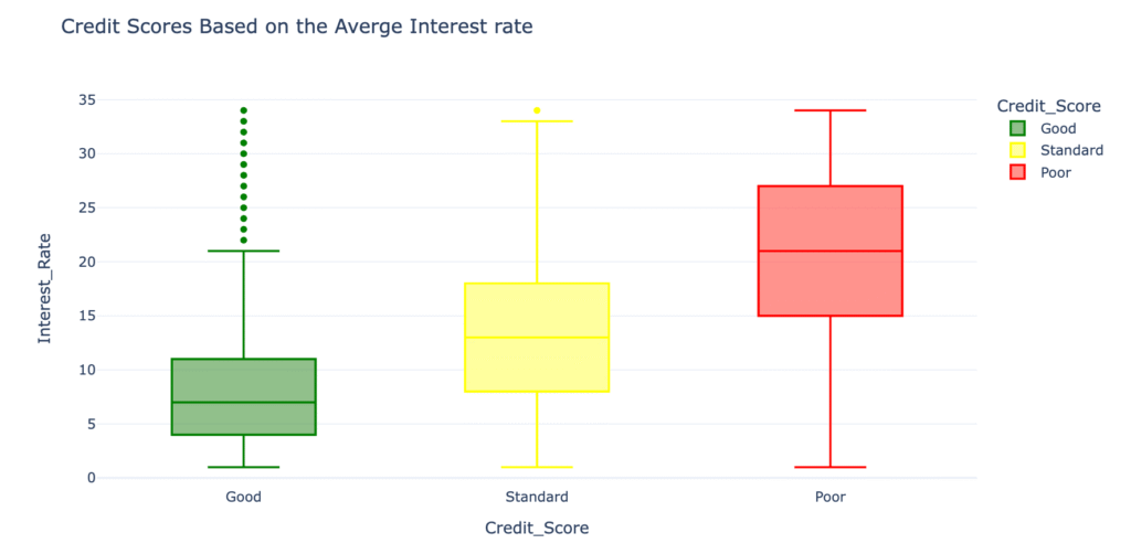
If the average interest rate is 4 – 11%, the credit score is good. Having an average interest rate of more than 15% is bad for your credit scores.
Now, let’s see how many loans you can take at a time for a good credit score:
fig=px.box(data,
           x="Credit_Score",
           y="Num_of_Loan",
           color="Credit_Score",
           title="Credit Scores Based on Number of Loans Taken by the Person",
           color_discrete_map={'Poor':'red',
                              'Standard':'yellow',
                              'Good':'green'})
fig.update_traces(quartilemethod="exclusive")
fig.show()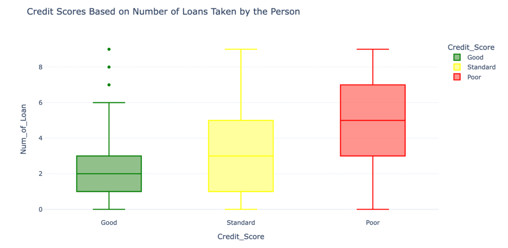
To have a good credit score, you should not take more than 1 – 3 loans at a time. Having more than three loans at a time will negatively impact your credit scores.
Now let’s see if delaying payments on the due date impacts your credit scores or not:
fig=px.box(data,
          x="Credit_Score",
          y="Delay_from_due_date",
          color="Credit_Score",
          title="Credit Score Based on Average Number of Days Delayed for Credit Card Payments",
          color_discrete_map={'Poor':'red',
                            'Standard':'yellow',
                            'Good':'green'})
fig.update_traces(quartilemethod="exclusive")
fig.show()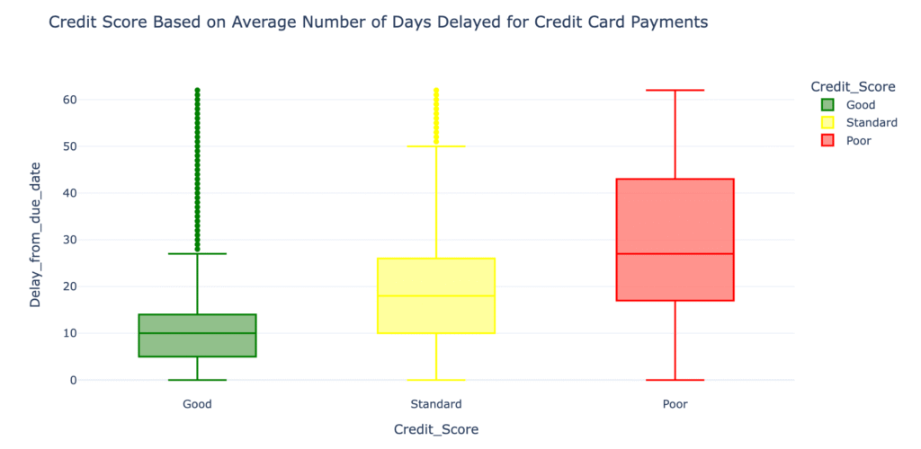
So you can delay your credit card payment 5 – 14 days from the due date. Delaying your payments for more than 17 days from the due date will impact your credit scores negatively.
Now, let’s have a look at whether frequently delaying payments will impact credit scores or not:
fig=px.box(data,
          x="Credit_Score",
          y="Num_of_Delayed_Payment",
          color="Credit_Score",
          title="Credit Scores Based on Delayed Payment",
          color_discrete_map={'Poor':'red',
                             'Standard':'yellow',
                             'Good':'green'})
fig.update_traces(quartilemethod="exclusive")
fig.show()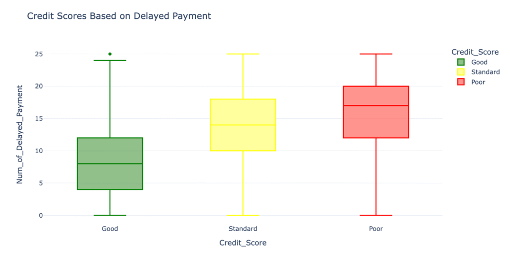
Delaying 4 – 12 payments from the due date will not affect your credit scores. But delaying more than 12 payments from the due date will affect your credit scores negatively.
Now let’s see if having more debt will affect credit scores or not:
fig=px.box(data,
          x="Credit_Score",
          y="Outstanding_Debt",
          color="Credit_Score",
          title="Credit Scores Based on Outstanding Debt",
          color_discrete_map={'Poor':'red',
                             'Standard':'yellow',
                             'Good':'green'})
fig.update_traces(quartilemethod="exclusive")
fig.show()
An outstanding debt of $380 – $1150 will not affect your credit scores. But always having a debt of more than $1338 will affect your credit scores negatively.
Now let’s see if having a high credit utilisation ratio will affect credit scores or not:
fig=px.box(data,
          x="Credit_Score",
          y="Credit_Utilization_Ratio",
          color="Credit_Score",
          title="Credit Scores Based on Credit Utilization Ratio",
          color_discrete_map={'Poor':'red',
                             'Standard':'yellow',
                             'Good':'green'})
fig.update_traces(quartilemethod="exclusive")
fig.show()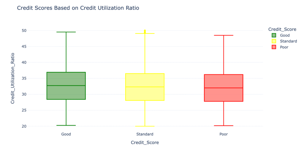
The credit utilization ratio means your total debt divided by your total available credit. According to the above plot, your credit utilization ratio doesn’t affect your credit scores.
Now, let’s see how the credit history age of a person affects credit scores:
fig=px.box(data,
          x="Credit_Score",
          y="Credit_History_Age",
          color="Credit_Score",
          title="Credit Scores Based on Credit History Age",
          color_discrete_map={'Poor':'red',
                             'Standard':'yellow',
                             'Good':'green'})
fig.update_traces(quartilemethod="exclusive")
fig.show()
So, having a long credit history results in better credit scores.
Now let’s see how many EMIs you can have in a month for a good credit score:
fig=px.box(data,
          x="Credit_Score",
          y="Total_EMI_per_month",
          color="Credit_Score",
          title="Credit Scores Based on Total Number of EMIs Per Month",
          color_discrete_map={'Poor':'red',
                             'Standard':'yellow',
                             'Good':'green'})
fig.update_traces(quartilemethod="exclusive")
fig.show()
The number of EMIs you are paying in a month doesn’t affect much on credit scores.
Now let’s see if your monthly investments affect your credit scores or not:
fig=px.box(data,
          x="Credit_Score",
          y="Amount_invested_monthly",
          color="Credit_Score",
          title="Credit Scores Based on Amount Invested Montly",
          color_discrete_map={'Poor':'red',
                             'Standard':'yellow',
                             'Good':'green'})
fig.update_traces(quartilemethod="exclusive")
fig.show()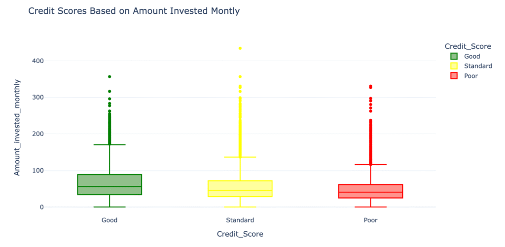
The amount of money you invest monthly doesn’t affect your credit scores a lot.
Now let’s see if having a low amount at the end of the month affects credit scores or not:
fig=px.box(data,
          x="Credit_Score",
          y="Monthly_Balance",
          color="Credit_Score",
          title="Credit Scores Based on Monthly Balance Left",
          color_discrete_map={'Poor':'red',
                             'Standard':'yellow',
                             'Good':'green'})
fig.update_traces(quartilemethod="exclusive")
fig.show()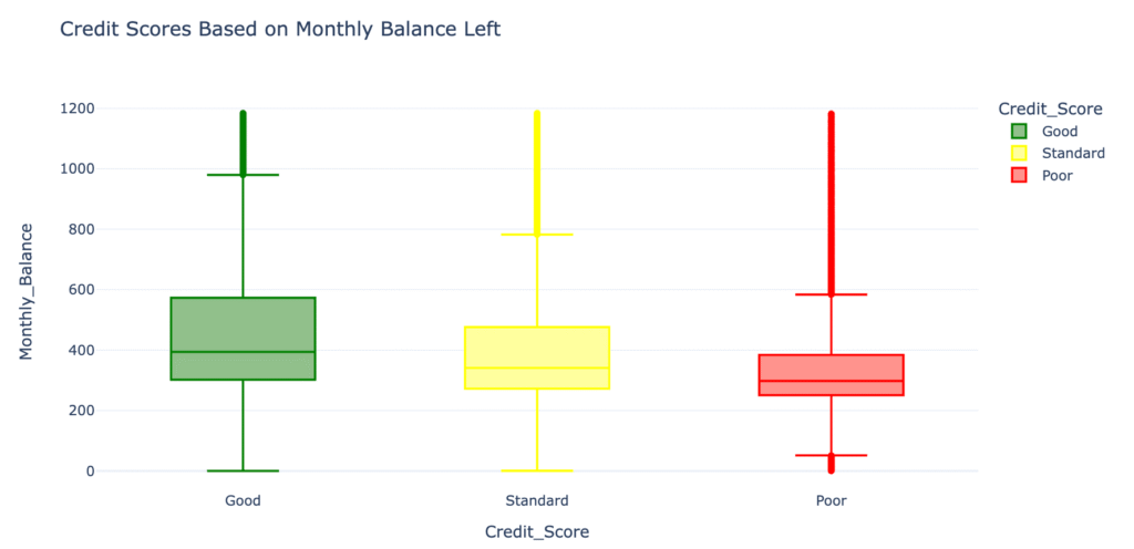
So, having a high monthly balance in your account at the end of the month is good for your credit scores. A monthly balance of less than $250 is bad for credit scores.
Credit Score Classification Model
An important feature in the dataset, Credit Mix, plays a key role in determining credit scores. It provides insights into the variety of credit and loan types a person has used.
Since the Credit_Mix column contains categorical data, I will convert it into a numerical format. This transformation is necessary to include it as an input for training a Machine Learning model for credit score classification.
data["Credit_Mix"] = data["Credit_Mix"].map({"Standard":1,
                                            "Good":2,
                                            "Bad":0})
Let’s split the data into features and labels by selecting the most relevant features for our model.
from sklearn.model_selection import train_test_split
x=np.array(data[["Annual_Income", "Monthly_Inhand_Salary",
                "Num_Bank_Accounts", "Num_Credit_Card",
                "Interest_Rate", "Num_of_Loan",
                "Delay_from_due_date", "Num_of_Delayed_Payment",
                "Credit_Mix", "Outstanding_Debt",
                "Credit_History_Age", "Monthly_Balance"]])
y=np.array(data[["Credit_Score"]])
Now, let’s split the data into training and test sets and proceed further by training a credit score classification model:
xtrain, xtest, ytrain, ytest=train_test_split(x, y, test_size=0.33, random_state=42)

from sklearn.ensemble import RandomForestClassifier
model = RandomForestClassifier()
model.fit(xtrain, ytrain)
Now, let’s make predictions from our model by giving inputs to our model according to the features we used to train the model:
print("Credit Score Prediction : ")
a= float(input("Annual Income: "))
b= float(input("Monthly Inhand Salary: "))
c= float(input("Number of Bank Accounts: "))
d= float(input("Number of Credit Cards: "))
e= float(input("Interest Rate: "))
f= float(input("Number of Loans: "))
g= float(input("Average Number of Days Delayed by the Person: "))
h= float(input("Number of Delayed Payments: "))
i= input("Credit Mix (Bad: 0, Standard: 1, Good: 3) : ")
j= float(input("Outstanding Debt: " ))
k= float(input("Credit History Age: "))
l= float(input("Monthly Balance: "))

features= np.array([[a, b, c, d, e, f, g, h, i, j, k, l]])
print("Predicted Credit Score = ", model.predict(features))
Conclusion
In this project, we used machine learning to classify credit scores into Good, Standard, and Poor, analyzing factors like income, debt, repayment history, and credit utilization. Our findings showed that higher income, timely payments, and a balanced credit mix strongly correlate with better scores, while excessive debt and frequent delays lower them.
The credit mix proved to be a key predictor, and converting categorical data to numerical form enhanced model accuracy. Future improvements could include testing advanced algorithms, fine-tuning parameters, or expanding the dataset with additional behavioral indicators.
If you’re interested in seeing how similar techniques apply to other fields, explore our Instagram Reach Analysis to learn how data science drives social media insights.
