
Predicting health insurance premiums has become one of the most practical applications of machine learning in the insurance industry. By analyzing various demographic and lifestyle factors such as age, BMI, smoking habits, and region we can build models that estimate how much a person might pay for health insurance.
In this project, we’ll walk through a complete workflow for health insurance premium prediction using Python and a Random Forest Regressor.
1. Importing Libraries
We’ll begin by importing essential libraries and connecting Google Drive to access the dataset.
from google.colab import drive
drive.mount('/content/drive')

file_id="1sbexs5rHN43HAZ3SLjg7-rFhVKgGAz8d"
url=f"https://drive.google.com/uc?id={file_id}"

import pandas as pd
import numpy as np
data=pd.read_csv(url)
The dataset that we are using for the task of health insurance premium prediction is collected from Kaggle. You can download the dataset from here. The dataset includes the following columns:
- age – Age of the person
- sex – Gender (male/female)
- bmi – Body Mass Index
- children – Number of dependents
- smoker – Whether the person smokes or not
- region – Residential region
- charges – The insurance premium (target variable)
2. Exploring the Dataset
Before building the model, it’s important to understand the structure of the data.
print(data.head())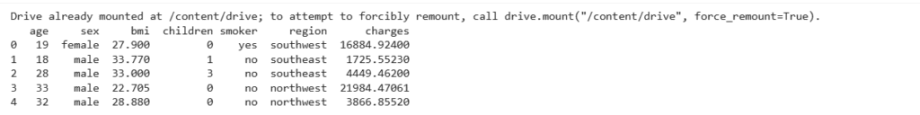
data.info()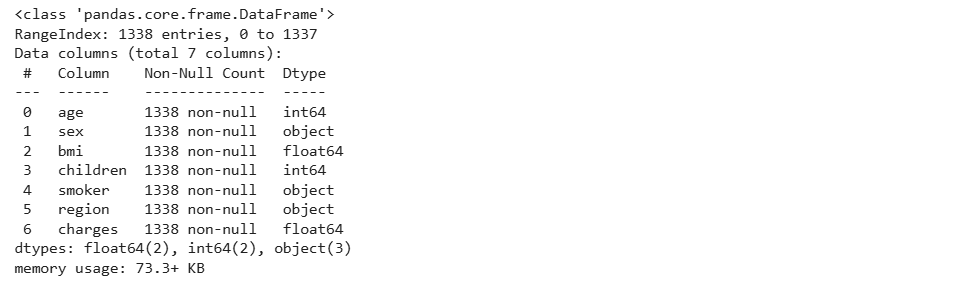
print(data.isnull().sum())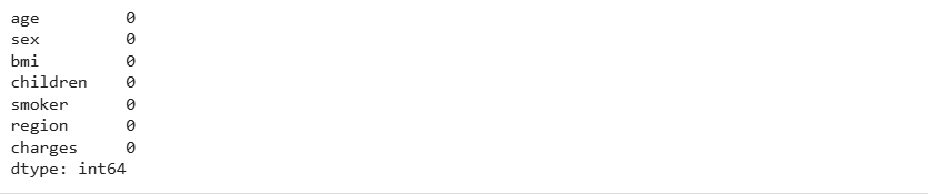
This helps us confirm there are no missing values and all columns are in the correct data type.
3. Visualizing the Data
We observed the “smoker” column, which indicates whether an individual is a smoker or not. This feature is particularly important, as smokers are generally more prone to major health issues compared to non-smokers. Let’s visualize the distribution of smokers and non-smokers in the dataset. We use Plotly Express for interactive and beautiful charts.
import plotly.express as px
data = data
figure = px.histogram(data, x = "sex",
                        color = "smoker",
                        title= "Number of Smokers",
                        text_auto=True)
figure.show()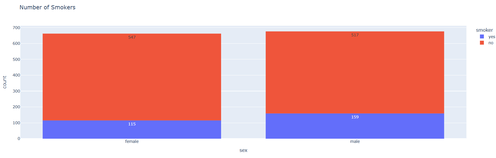
Interpretation: According to the visualization above, 547 females and 517 males are non-smokers, while 115 females and 159 males are smokers. Now, let’s explore the distribution of the regions where individuals in the dataset reside:
import plotly.express as px
pie = data["region"].value_counts()
regions = pie.index
population = pie.values
fig = px.pie(data, values=population, names=regions, title="Region Distribution")
fig.show()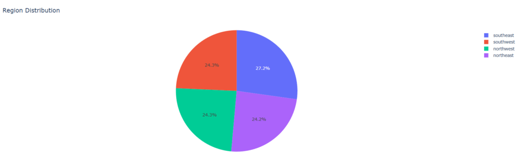
4. Data Preprocessing and Encoding
Machine learning models require numerical data, so we’ll convert categorical variables into numeric form.
data["sex"] = data["sex"].map({"female": 0, "male": 1})
data["smoker"] = data["smoker"].map({"no": 0, "yes": 1})
print(data.head())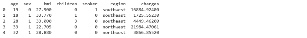
data = pd.get_dummies(data, columns=["region"], drop_first=True)
print(data.head())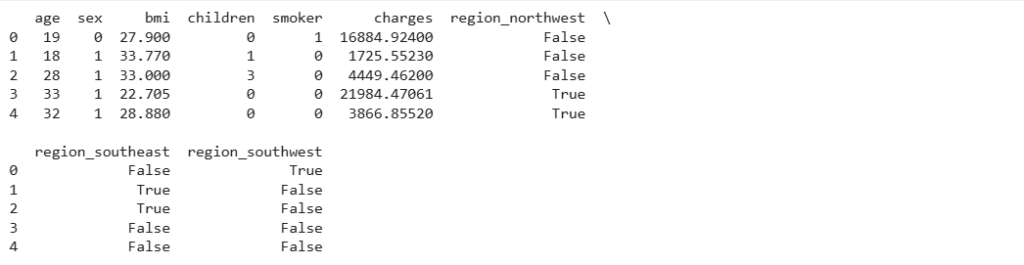
We used one-hot encoding for the region feature since it has multiple categories. Now, let’s examine the correlation between the features in this dataset:
print(data.corr())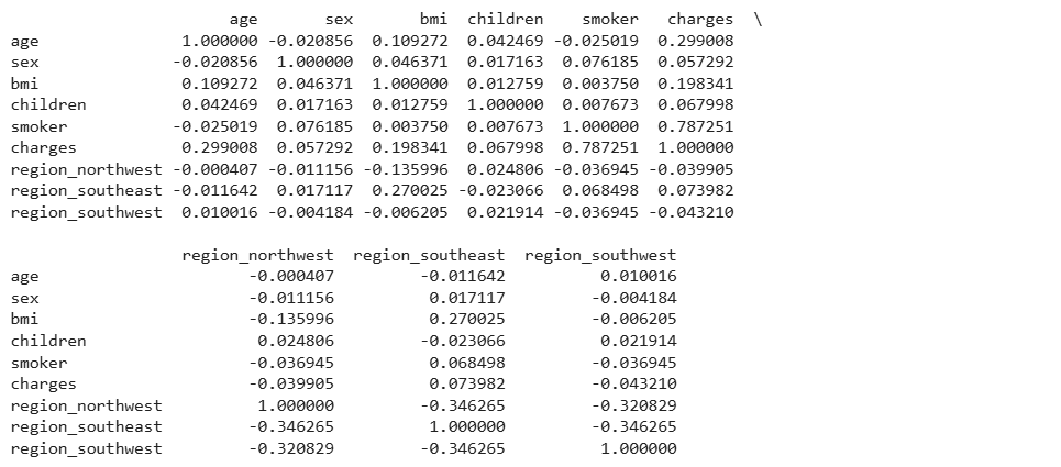
5. Splitting the Data
Now let’s separate the data into features (X) and target (y), and split them into training and test sets.
x = data.drop("charges", axis=1)
y = data["charges"]

from sklearn.model_selection import train_test_split
xtrain, xtest, ytrain, ytest = train_test_split(x, y, test_size=0.2, random_state=42)
This ensures 80% of data is used for training and 20% for testing.
6. Building the Random Forest Model
We’ll use a Random Forest Regressor, a powerful ensemble learning algorithm that handles non-linear relationships effectively.
from sklearn.ensemble import RandomForestRegressor
forest = RandomForestRegressor(random_state=42)
forest.fit(xtrain, ytrain)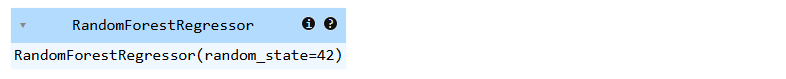
The model learns the relationship between input features and insurance charges.
7. Making Predictions
After training, let’s make predictions on the test set:
ypred = forest.predict(xtest)To visualize or inspect, we create a small comparison table:
pred_data = pd.DataFrame({"Actual": ytest, "Predicted": ypred})
print(pred_data.head())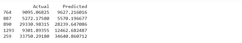
8. Evaluating the Model
To check the model’s performance, we need to calculate R² Score, Mean Absolute Error (MAE), and Root Mean Squared Error (RMSE).
from sklearn.metrics import r2_score, mean_absolute_error, mean_squared_error

r2 = r2_score(ytest, ypred)
mae = mean_absolute_error(ytest, ypred)
mse = mean_squared_error(ytest, ypred)   # always available
rmse = np.sqrt(mse)                      # root of MSE

print(f"R² Score: {r2:.3f}")
print(f"MAE: {mae:.2f}")
print(f"RMSE: {rmse:.2f}")
These values show how accurately the model predicts premium amounts compared to actual values.
9. Analyzing Feature Importance
Random Forests allow us to inspect which features influence predictions the most.
import matplotlib.pyplot as plt

importances = forest.feature_importances_
features = x.columns
plt.barh(features, importances)
plt.title("Feature Importance in Premium Prediction")
plt.xlabel("Importance")
plt.ylabel("Feature")
plt.show()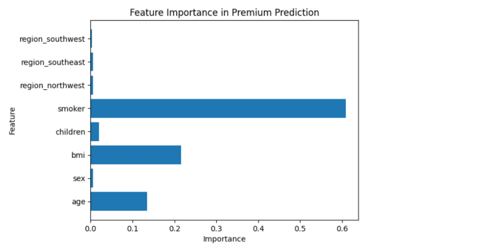
🩺 Typically, smoking status, BMI, and age are the most significant predictors of insurance premium costs.
Conclusion
This project demonstrates how machine learning can predict health insurance premiums based on demographic and lifestyle factors. The Random Forest model provides strong performance out of the box and is interpretable enough for exploratory analysis.
Key Takeaways
- Machine learning models can effectively estimate premium costs when given the right inputs.
- Categorical encoding and proper data preprocessing are crucial.
- Model evaluation using metrics like MAE and RMSE helps validate accuracy.
- Insights from feature importance can help insurers understand key cost drivers.
By using machine learning, insurers and data scientists can create smarter, data-driven tools for health insurance pricing. Just as algorithms used in food delivery time prediction help estimate arrival times based on multiple factors, predictive models in insurance make pricing more accurate while promoting fairness and transparency in premium calculations.